Data cleaning & transformation with dplyr
Last updated on 2026-04-21 | Edit this page
Overview
Questions
- How can I create new columns or remove exisitng columns from a data frame?
- How can I rename variables or assign new values to a variable?
- How can I combine multiple commands into a single command?
- How can I export my data frame to a csv file?
Objectives
- Describe the functions available in the
dplyrandtidyrpackages. - Recognise and use the following functions:
select(),filter(),rename(),recode(),mutate()andarrange(). - Combine one or more functions using the ‘pipe’ operator
%>%. - Use the split-apply-combine concept for data analysis.
- Export a data frame to a csv file.
Transforming data with dplyr
We are now entering the data cleaning and transforming phase. While
it is possible to do much of the following using Base R functions (in
other words, without loading an external package) dplyr
makes it much easier. Like many of the most useful R packages,
dplyr was developed by data scientist http://hadley.nz/.
dplyr is a package for making tabular data manipulation
easier by using a limited set of functions that can be combined to
extract and summarize insights from your data. It pairs nicely with
tidyr which enables you to swiftly convert
between different data formats (long vs. wide) for plotting and
analysis.
dplyr is also part of the tidyverse. Let’s
make sure we are all on the same page by loading the
tidyverse and the books dataset we downloaded
earlier.
We’re going to learn some of the most common
dplyr functions:
-
rename(): rename columns -
recode(): recode values in a column -
select(): subset columns -
filter(): subset rows on conditions -
mutate(): create new columns by using information from other columns -
group_by()andsummarize(): create summary statistics on grouped data -
arrange(): sort results -
count(): count discrete values
Getting set up
Make sure you have your Rproj and directories set up from the previous episode.
If you have not completed that step, run the following in your Rproj:
R
library(fs)   # https://fs.r-lib.org/.  fs is a cross-platform, uniform interface to file system operations via R.
dir_create("data")
dir_create("data_output")
dir_create("fig_output")
download.file("https://ndownloader.figshare.com/files/22031487",
              "data/books.csv", mode = "wb")
Then load the tidyverse package
R
library(tidyverse)
OUTPUT
── Attaching core tidyverse packages ──────────────────────── tidyverse 2.0.0 ──
✔ dplyr     1.2.1     ✔ purrr     1.2.1
✔ forcats   1.0.1     ✔ stringr   1.6.0
✔ ggplot2   4.0.2     ✔ tibble    3.3.1
✔ lubridate 1.9.5     ✔ tidyr     1.3.2
── Conflicts ────────────────────────────────────────── tidyverse_conflicts() ──
✖ dplyr::filter() masks stats::filter()
✖ dplyr::lag()    masks stats::lag()
ℹ Use the conflicted package (<http://conflicted.r-lib.org/>) to force all conflicts to become errors
and the books data we saved in the previous lesson.
R
books <- read_csv("data/books.csv") # load the data and assign it to books
Renaming variables
It is often necessary to rename variables to make them more
meaningful. If you print the names of the sample books
dataset you can see that some of the vector names are not particularly
helpful:
R
glimpse(books) # print names of the books data frame to the console
OUTPUT
Rows: 10,000
Columns: 12
$ CALL...BIBLIO. <chr> "001.94 Don 2000", "001.942 Bro 1999", "027.073 App 200…
$ X245.ab        <chr> "Bermuda Triangle /", "Invaders from outer space :|real…
$ X245.c         <chr> "written by Andrew Donkin.", "written by Philip Brooks.…
$ LOCATION       <chr> "juv", "juv", "juv", "juv", "juv", "juv", "juv", "juv",…
$ TOT.CHKOUT     <dbl> 6, 2, 3, 6, 7, 6, 4, 2, 4, 13, 6, 7, 3, 22, 2, 9, 4, 8,…
$ LOUTDATE       <chr> "11-21-2013 9:44", "02-07-2004 15:29", "10-16-2007 10:5…
$ SUBJECT        <chr> "Readers (Elementary)|Bermuda Triangle -- Juvenile lite…
$ ISN            <chr> "0789454165 (hbk.)~0789454157 (pbk.)", "0789439999 (har…
$ CALL...ITEM.   <chr> "001.94 Don 2000", "001.942 Bro 1999", "027.073 App 200…
$ X008.Date.One  <chr> "2000", "1999", "2001", "1999", "2000", "2001", "2001",…
$ BCODE2         <chr> "a", "a", "a", "a", "a", "a", "a", "a", "a", "a", "a", …
$ BCODE1         <chr> "j", "j", "j", "j", "j", "j", "j", "j", "j", "j", "j", …
There are many ways to rename variables in R, but the
rename() function in the dplyr package is the
easiest and most straightforward. The new variable name comes first. See
help(rename).
Here we rename the X245.ab variable. Make sure you assign the output
to your books value, otherwise it will just print it to the
console. In other words, we are overwriting the previous
books value with the new one, with X245.ab
renamed to title.
R
# rename the . Make sure you return (<-) the output to your
# variable, otherwise it will just print it to the console
books <- rename(books,
                title = X245.ab)
Tip:
When using the rename() function, the new variable name
comes first.
Side note:
Where does X245.ab come from? That is the MARC field
245|ab. However, because R variables cannot start with a number, R
automatically inserted an X, and because pipes | are not allowed in
variable names, R replaced it with a period.
You can also rename multiple variables at once by running:
R
# rename multiple variables at once
books <- rename(books,
                author = X245.c,
                callnumber = CALL...BIBLIO.,
                isbn = ISN,
                pubyear = X008.Date.One,
                subCollection = BCODE1,
                format = BCODE2,
                location = LOCATION,
                tot_chkout = TOT.CHKOUT,
                loutdate = LOUTDATE,
                subject = SUBJECT)
books
OUTPUT
# A tibble: 10,000 × 12
   callnumber        title     author location tot_chkout loutdate subject isbn
   <chr>             <chr>     <chr>  <chr>         <dbl> <chr>    <chr>   <chr>
 1 001.94 Don 2000   Bermuda … writt… juv               6 11-21-2… Reader… 0789…
 2 001.942 Bro 1999  Invaders… writt… juv               2 02-07-2… Reader… 0789…
 3 027.073 App 2001  Down Cut… by Ka… juv               3 10-16-2… Packho… 0060…
 4 133.5 Hua 1999    The Chin… by Ch… juv               6 11-22-2… Astrol… 0060…
 5 170 She 2000      Judge Ju… illus… juv               7 04-10-2… Childr… 0060…
 6 170.44 She 2001   Judge Ju… illus… juv               6 11-12-2… Conduc… 0060…
 7 220.9505 Gil 2001 A young … retol… juv               4 12-01-2… Bible … 0060…
 8 225.9505 McC 1999 God's Ki… retol… juv               2 08-06-2… Bible … 0689…
 9 292.13 McC 2001   Roman my… retol… juv               4 04-03-2… Mythol… 0689…
10 292.211 McC 1998  Greek go… retol… juv              13 11-16-2… Gods, … 0689…
# ℹ 9,990 more rows
# ℹ 4 more variables: CALL...ITEM. <chr>, pubyear <chr>, format <chr>,
# subCollection <chr>Rename CALL...ITEM.
- Use
rename()to rename theCALL...ITEM.column tocallnumber2. Remember to add the period to the end of theCALL...ITEM.value
R
books <- rename(books,
                callnumber2 = CALL...ITEM.)
Recoding values
It is often necessary to recode or reclassify values in your data.
For example, in the sample dataset provided to you, the
sub_collection (formerly BCODE1) and
format (formerly BCODE2) variables contain
single characters.
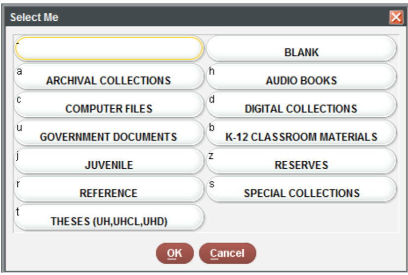
You can reassign names to the values easily using the
recode() function from the dplyr package.
Unlike rename(), the old value comes first here. Also
notice that we are overwriting the books$subCollection
variable.
R
# first print to the console all of the unique values you will need to recode
distinct(books, subCollection)
OUTPUT
FALSE # A tibble: 10 × 1
FALSE    subCollection
FALSE    <chr>
FALSE  1 j
FALSE  2 b
FALSE  3 u
FALSE  4 r
FALSE  5 -
FALSE  6 s
FALSE  7 c
FALSE  8 z
FALSE  9 a
FALSE 10 t
R
books$subCollection <- recode(books$subCollection,
                                      "-" = "general collection",
                                      u = "government documents",
                                      r = "reference",
                                      b = "k-12 materials",
                                      j = "juvenile",
                                      s = "special collections",
                                      c = "computer files",
                                      t = "theses",
                                      a = "archives",
                                      z = "reserves")
books
OUTPUT
FALSE # A tibble: 10,000 × 12
FALSE callnumber title author location tot_chkout loutdate subject isbn
FALSE <chr> <chr> <chr> <chr> <dbl> <chr> <chr> <chr>
FALSE 1 001.94 Don 2000 Bermuda … writt… juv 6 11-21-2… Reader… 0789…
FALSE 2 001.942 Bro 1999 Invaders… writt… juv 2 02-07-2… Reader… 0789…
FALSE 3 027.073 App 2001 Down Cut… by Ka… juv 3 10-16-2… Packho… 0060…
FALSE 4 133.5 Hua 1999 The Chin… by Ch… juv 6 11-22-2… Astrol… 0060…
FALSE 5 170 She 2000 Judge Ju… illus… juv 7 04-10-2… Childr… 0060…
FALSE 6 170.44 She 2001 Judge Ju… illus… juv 6 11-12-2… Conduc… 0060…
FALSE 7 220.9505 Gil 2001 A young … retol… juv 4 12-01-2… Bible … 0060…
FALSE 8 225.9505 McC 1999 God's Ki… retol… juv 2 08-06-2… Bible … 0689…
FALSE 9 292.13 McC 2001 Roman my… retol… juv 4 04-03-2… Mythol… 0689…
FALSE 10 292.211 McC 1998 Greek go… retol… juv 13 11-16-2… Gods, … 0689…
FALSE # ℹ 9,990 more rows
FALSE # ℹ 4 more variables: callnumber2 <chr>, pubyear <chr>, format <chr>,
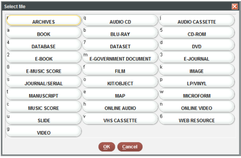
FALSE # subCollection <chr>Do the same for the format column. Note that you must
put "5" and "4" into quotation marks for the
function to operate correctly.
R
books$format <- recode(books$format,
                              a = "book",
                              e = "serial",
                              w = "microform",
                              s = "e-gov doc",
                              o = "map",
                              n = "database",
                              k = "cd-rom",
                              m = "image",
                              "5" = "kit/object",
                              "4" = "online video")
Once you have finished recoding the values for the two variables, examine the dataset again and check to see if you have different values this time:
R
distinct(books, subCollection, format)
Subsetting dataframes
Subset rows with filter()
In the last lesson we learned how to subset a data frame using
brackets. As with other R functions, the dplyr package
makes it much more straightforward, using the filter()
function.
Here we will create a subset of books called
booksOnly, which includes only those items where the format
is books. Notice that we use two equal signs == as the
logical operator:
R
booksOnly <- filter(books, format == "book") # filter books to return only those items where the format is books
You can also use multiple filter conditions. Here, the order matters: first we filter to include only books, then of the results, we include only items that have more than zero checkouts.
R
bookCheckouts <- filter(books,
                        format == "book",
                        tot_chkout > 0)
How many items were removed? You can find out functionally with:
R
nrow(books) - nrow(bookCheckouts)
OUTPUT
FALSE [1] 5733You can then check the summary statistics of checkouts for books with more than zero checkouts. Notice how different these numbers are from the previous lesson, when we kept zero in. The median is now 3 and the mean is 5.
R
summary(bookCheckouts$tot_chkout)
OUTPUT
FALSE    Min. 1st Qu.  Median    Mean 3rd Qu.    Max.
FALSE   1.000   2.000   3.000   5.281   6.000 113.000
If you want to filter on multiple conditions within the same
variable, use the %in% operator combined with a vector of
all the values you wish to include within c(). For example,
you may want to include only items in the format serial and
microform:
R
serial_microform <- filter(books, format %in% c("serial", "microform"))
Exercise: Subsetting with
filter()
Use
filter()to create a data frame calledbooksJuvconsisting offormatbooks andsubCollectionjuvenile materials.Use
mean()to check the average number of checkouts for thebooksJuvdata frame.
R
booksJuv <- filter(books,
               format == "book",
               subCollection ==  "juvenile")
mean(booksJuv$tot_chkout)
OUTPUT
[1] 10.41404Subset columns with select()
The select() function allows you to keep or remove
specific columns It also provides a convenient way to reorder
variables.
R
# specify the variables you want to keep by name
booksTitleCheckouts <- select(books, title, tot_chkout)
booksTitleCheckouts
OUTPUT
# A tibble: 10,000 × 2
   title                                                              tot_chkout
   <chr>                                                                   <dbl>
 1 Bermuda Triangle /                                                          6
 2 Invaders from outer space :|real-life stories of UFOs /                     2
 3 Down Cut Shin Creek :|the pack horse librarians of Kentucky /               3
 4 The Chinese book of animal powers /                                         6
 5 Judge Judy Sheindlin's Win or lose by how you choose! /                     7
 6 Judge Judy Sheindlin's You can't judge a book by its cover :|cool…          6
 7 A young child's Bible /                                                     4
 8 God's Kingdom :|stories from the New Testament /                            2
 9 Roman myths /                                                               4
10 Greek gods and goddesses /                                                 13
# ℹ 9,990 more rows
R
# specify the variables you want to remove with a -
books <- select(books, -location)

# reorder columns, combined with everything()
booksReordered <- select(books, title, tot_chkout, loutdate, everything())
Tips:
If your variable name has spaces, use `` to close the variable:
R
select(df, -`my variable`)
ERROR
Error in `UseMethod()`:
! no applicable method for 'select' applied to an object of class "function"
Ordering data with arrange()
The arrange() function in the dplyr package
allows you to sort your data by alphabetical or numerical order.
R
booksTitleArrange <- arrange(books, title)

# use desc() to sort a variable in descending order
booksHighestChkout <- arrange(books, desc(tot_chkout))
booksHighestChkout
OUTPUT
# A tibble: 10,000 × 11
   callnumber title author tot_chkout loutdate subject isbn  callnumber2 pubyear
   <chr>      <chr> <chr>       <dbl> <chr>    <chr>   <chr> <chr>       <chr>
 1 E Cro 2000 Clic… by Do…        113 01-23-2… Cows -… 0689… E Cro 2000  2000
 2 PZ7.W6367… The … by Da…        106 03-07-2… Pigs -… 0618… 398.2452 W… 2001
 3 <NA>       Cook… Janet…        103 03-13-2… Cake -… 0152… E Ste 1999  1999
 4 PZ7.D5455… Beca… Kate …         79 03-27-2… Dogs -… 0763… Fic Dic 20… 2000
 5 PZ7.C6775… Upto… Bryan…         69 02-05-2… Harlem… 9780… E Col 2000  2000
 6 <NA>       <NA>  <NA>           64 08-23-2… <NA>    <NA>  #1  ENC. C… <NA>
 7 F379.N59 … Thro… Ruby …         63 11-01-2… Bridge… 0590… 920 Bri 19… 1999
 8 PZ7.C9413… Bud,… Chris…         63 04-03-2… Runawa… 0385… Fic Cur 19… 1999
 9 E Mar 1992 Brow… by Bi…         61 02-16-2… Color … 0805… E Mar 1992  1992
10 PZ7.P338 … A ye… Richa…         47 03-26-2… Grandm… 0803… Fic Pec 20… 2000
# ℹ 9,990 more rows
# ℹ 2 more variables: format <chr>, subCollection <chr>
R
# order data based on multiple variables (e.g. sort first by checkout, then by publication year)
booksChkoutYear <- arrange(books, desc(tot_chkout), desc(pubyear))
Creating new variables with mutate()
The mutate() function allows you to create new
variables. Here, we use the str_sub() function from the
stringr package to extract the first character of the
callnumber variable (the call number class) and put it into
a new column called call_class.
R
booksLC <- mutate(books,
                  call_class = str_sub(callnumber, 1, 1))
There are two numbers because you must specify a start and an end value–here, we start with the first character, and end with the first character.
mutate() is also helpful to coerce a column from one
data type to another. For example, we can see there are some errors in
the pubyear variable–some dates are 19zz or
uuuu. As a result, this variable was read in as a
character rather than an integer.
R
books <- mutate(books, pubyear = as.integer(pubyear))
WARNING
Warning: There was 1 warning in `mutate()`.
ℹ In argument: `pubyear = as.integer(pubyear)`.
Caused by warning:
! NAs introduced by coercion
We see the error message NAs introduced by coercion.
This is because non-numerical variables become NA and the
remainder become integers.
Putting it all together with %>%
The Pipe
Operator %>% is loaded with the
tidyverse. It takes the output of one statement and makes
it the input of the next statement. You can think of it as “then” in
natural language. So instead of making a bunch of intermediate data
frames and cluttering up your workspace, you can run multiple functions
at once. You can type the pipe with Ctrl + Shift +
M if you have a PC or Cmd + Shift +
M if you have a Mac.
So in the following example, the books tibble is first
called, then the format is filtered to include only
book, then only the title and
tot_chkout columns are selected, and finally the data is
rearranged from most to least checkouts.
R
myBooks <- books %>%
  filter(format == "book") %>%
  select(title, tot_chkout) %>%
  arrange(desc(tot_chkout))
myBooks
OUTPUT
# A tibble: 6,983 × 2
   title                                      tot_chkout
   <chr>                                           <dbl>
 1 Click, clack, moo :|cows that type /              113
 2 The three pigs /                                  106
 3 Cook-a-doodle-doo! /                              103
 4 Because of Winn-Dixie /                            79
 5 Uptown /                                           69
 6 Through my eyes /                                  63
 7 Bud, not Buddy /                                   63
 8 Brown bear, brown bear, what do you see? /         61
 9 A year down yonder /                               47
10 Wemberly worried /                                 43
# ℹ 6,973 more rowsExercise: Playing with pipes
%>%
- Create a new data frame
booksKidswith these conditions:
-
filter()to includesubCollectionjuvenile & k-12 materials andformatbooks. -
select()only title, call number, total checkouts, and publication year -
arrange()by total checkouts in descending order
- Use
mean()to check the average number of checkouts for thebooksKidsdata frame.
R
booksKids <- books %>%
  filter(subCollection %in% c("juvenile", "k-12 materials"),
  format == "book") %>%
select(title, callnumber, tot_chkout, pubyear) %>%
arrange(desc(tot_chkout))
mean(booksKids$tot_chkout)
OUTPUT
[1] 9.336331Split-apply-combine and the summarize() function
Many data analysis tasks can be approached using the
split-apply-combine paradigm: split the data into groups, apply
some analysis to each group, and then combine the results.
dplyr makes this very easy through the use
of the group_by() function.
The summarize() function
group_by() is often used together with
summarize(), which collapses each group into a single-row
summary of that group. group_by() takes as arguments the
column names that contain the categorical variables for
which you want to calculate the summary statistics.
So to compute the average checkouts by format:
R
books %>%
  group_by(format) %>%
  summarize(mean_checkouts = mean(tot_chkout))
OUTPUT
# A tibble: 10 × 2
   format       mean_checkouts
   <chr>                 <dbl>
 1 book                3.23
 2 cd-rom              0.333
 3 database            0
 4 e-gov doc           0.0402
 5 image               0.0275
 6 kit/object          1.33
 7 map                10.6
 8 microform           0.00122
 9 online video        0
10 serial              0
Books and maps have the highest, and as we would expect, databases, online videos, and serials have zero checkouts.
Here is a more complex example:
R
books %>%
  filter(format == "book") %>%
  mutate(call_class = str_sub(callnumber, 1, 1)) %>%
  group_by(call_class) %>%
  summarize(count = n(),
            sum_tot_chkout = sum(tot_chkout)) %>%
  arrange(desc(sum_tot_chkout))
OUTPUT
# A tibble: 34 × 3
   call_class count sum_tot_chkout
   <chr>      <int>          <dbl>
 1 E            487           3114
 2 <NA>         459           3024
 3 H           1142           2902
 4 P            800           2645
 5 F            240           1306
 6 Q            333           1305
 7 B            426           1233
 8 R            193            981
 9 L            358            862
10 5             60            838
# ℹ 24 more rows
Let’s break this down step by step:
- First we call the
booksdata frame - We then pipe through
filter()to include only books - We then create a new column with
mutate()calledcall_classby using thestr_sub()function to keep the first character of thecall_numbervariable - We then
group_by()our newly createdcall_classvariable - We then create two summary columns by using
summarize()- take the number
n()of items percall_classand assign it to a column calledcount - take the the
sum()oftot_chkoutpercall_classand assign the result to a column calledsum_tot_chkout
- take the number
- Finally, we arrange
sum_tot_chkoutin descending order, so we can see the class with the most total checkouts. We can see it is theEclass (History of America), followed byNA(items with no call number data), followed byH(Social Sciences) andP(Language and Literature).
Pattern matching
Cleaning text with the stringr package is easier when
you have a basic understanding of ‘regex’, or regular expression pattern
matching. Regex is especially useful for manipulating strings
(alphanumeric data), and is the backbone of search-and-replace
operations in most applications. Pattern matching is common to all
programming languages but regex syntax is often code-language specific.
Below, find an example of using pattern matching to find and replace
data in R:
- Remove the trailing slash in the title column
- Modify the punctuation separating the title from a subtitle
Note: If the final product of this data will be imported into an ILS, you may not want to alter the MARC specific punctuation. All other audiences will appreciate the text normalizing steps.
Read more about matching patterns with regular expressions.
R
books %>%
  mutate(title_modified = str_remove(title, "/$")) %>%     # remove the trailing slash
  mutate(title_modified = str_replace(title_modified, "\\s:\\|", ": ")) %>%   # replace ' :|' with ': '
  select(title_modified, title)
OUTPUT
# A tibble: 10,000 × 2
   title_modified                                                          title
   <chr>                                                                   <chr>
 1 "Bermuda Triangle "                                                     Berm…
 2 "Invaders from outer space: real-life stories of UFOs "                 Inva…
 3 "Down Cut Shin Creek: the pack horse librarians of Kentucky "           Down…
 4 "The Chinese book of animal powers "                                    The …
 5 "Judge Judy Sheindlin's Win or lose by how you choose! "                Judg…
 6 "Judge Judy Sheindlin's You can't judge a book by its cover: cool rule… Judg…
 7 "A young child's Bible "                                                A yo…
 8 "God's Kingdom: stories from the New Testament "                        God'…
 9 "Roman myths "                                                          Roma…
10 "Greek gods and goddesses "                                             Gree…
# ℹ 9,990 more rows
Exporting data
Now that you have learned how to use
dplyr to extract information from or
summarize your raw data, you may want to export these new data sets to
share them with your collaborators or for archival.
Similar to the read_csv() function used for reading CSV
files into R, there is a write_csv() function that
generates CSV files from data frames.
We have previously created the directory data_output
which we will use to store our generated dataset. It is good practice to
keep your input and output data in separate folders–the
data folder should only contain the raw, unaltered data,
and should be left alone to make sure we don’t delete or modify it.
In preparation for our next lesson on plotting, we are going to create a version of the dataset with most of the changes we made above. We will first read in the original, then make all the changes with pipes.
R
books_reformatted <- read_csv("./data/books.csv") %>%
  rename(title = X245.ab,
         author = X245.c,
         callnumber = CALL...BIBLIO.,
         isbn = ISN,
         pubyear = X008.Date.One,
         subCollection = BCODE1,
         format = BCODE2,
         location = LOCATION,
         tot_chkout = TOT.CHKOUT,
         loutdate = LOUTDATE,
         subject = SUBJECT,
         callnumber2 = CALL...ITEM.) %>%
  mutate(pubyear = as.integer(pubyear),
         call_class = str_sub(callnumber, 1, 1),
         subCollection = recode(subCollection,
                                "-" = "general collection",
                                u = "government documents",
                                r = "reference",
                                b = "k-12 materials",
                                j = "juvenile",
                                s = "special collections",
                                c = "computer files",
                                t = "theses",
                                a = "archives",
                                z = "reserves"),
         format = recode(format,
                         a = "book",
                         e = "serial",
                         w = "microform",
                         s = "e-gov doc",
                         o = "map",
                         n = "database",
                         k = "cd-rom",
                         m = "image",
                         "5" = "kit/object",
                         "4" = "online video"))
This chunk of code read the CSV, renamed the variables, used
mutate() in combination with recode() to
recode the format and subCollection values,
used mutate() in combination with as.integer()
to coerce pubyear to integer, and used
mutate() in combination with str_sub to create
the new varable call_class.
We now write it to a CSV and put it in the data/output
sub-directory:
R
write_csv(books_reformatted, "./data_output/books_reformatted.csv")
Help with dplyr
- Read more about
dplyrat https://dplyr.tidyverse.org/. - In your console, after loading
library(dplyr), runvignette("dplyr")to read an extremely helpful explanation of how to use it. - See the http://r4ds.had.co.nz/transform.html in Garrett Grolemund and Hadley Wickham’s book R for Data Science.
- Watch this Data School video: https://www.youtube.com/watch?v=jWjqLW-u3hc
- Use the
dplyrpackage to manipulate dataframes. - Subset data frames using
select()andfilter(). - Rename variables in a data frame using
rename(). - Recode values in a data frame using
recode(). - Use
mutate()to create new variables. - Sort data using
arrange(). - Use
group_by()andsummarize()to work with subsets of data. - Use pipe (
%>%) to combine multiple commands.