Starting with Data

Overview

Questions

• What is a working directory?
• How can I create new sub-directories in R?
• How can I read a complete csv file into R?
• How can I get basic summary information about my dataset?
• How can I extract certain rows and columns from my data frame?
• How can I deal with missing values in R?

Objectives

• Set up the working directory and sub-directories.
• Load external data from a .csv file into a data frame.
• Describe what a data frame is.
• Summarize the contents of a data frame.
• Indexing and subsetting data frames.
• Explore missing values in data frames.
• Use logical operators in data frames.

Create a new R project

---

Let’s create a new project library_carpentry.Rproj in RStudio to play with our dataset.

Reminder

In the previous episode Before We Start, we briefly walk through how to create an R project to keep all your scripts, data and analysis. If you need a refreshment, go back to this episode and follow the instructions on creating an R project folder.

Once you have created the project, open the project in RStudio.

Getting data into R

---

We will be using a demo dataset from the University of Houston–Clear Lake Integrated Library System in 2018. It contains a relatively random sample of books from the catalog.

In order to use your data in R, you must import it and turn it into an R object. There are many ways to get data into R.

• Manually: You can manually create it using the data.frame() function in Base R, or the tibble() function in the tidyverse.

• Import it from a file Below is a very incomplete list

  • Text: TXT (readLines() function)
  • Tabular data: CSV, TSV (read.table() function or readr package)
  • Excel: XLSX (xlsx package)
  • Google sheets: (googlesheets package)
  • Statistics program: SPSS, SAS (haven package)
  • Databases: MySQL (RMySQL package)

• Gather it from the web: You can connect to webpages, servers, or APIs directly from within R, or you can create a data scraped from HTML webpages using the rvest package. For example

  • the Twitter API with twitteR
  • Crossref data with rcrossref
  • World Bank’s World Development Indicators with WDI.

Set up your working directory

The working directory is an important concept to understand. It is the place on your computer where R will look for and save files. When you write code for your project, your scripts should refer to files in relation to the root of your working directory and only to files within this structure. Using RStudio projects makes this easy and ensures that your working directory is set up properly.

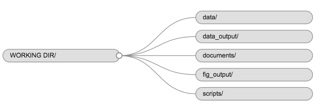
Using a consistent folder structure across your projects will help keep things organized and make it easy to find/file things in the future. This can be especially helpful when you have multiple projects. In general, you might create directories (folders) for scripts, data, and documents. Here are some examples of suggested directories:

• data/ Use this folder to store your raw data and intermediate datasets. For the sake of transparency and provenance, you should always keep a copy of your raw data accessible and do as much of your data cleanup and preprocessing programmatically (i.e., with scripts, rather than manually) as possible.
• data_output/ When you need to modify your raw data, it might be useful to store the modified versions of the datasets in a different folder.
• documents/ Used for outlines, drafts, and other text.
• fig_output/ This folder can store the graphics that are generated by your scripts.
• scripts/ A place to keep your R scripts for different analyses or plotting.

You may want additional directories or subdirectories depending on your project needs, but these should form the backbone of your working directory.

Using the getwd() and setwd() commands

Knowing your current directory is important so that you save your files, scripts and output in the right location. You can check your current directory by running getwd() in the RStudio interface. If for some reason your working directory is not what it should be, you can change it manually by navigating in the file browser to where your working directory should be, then by clicking on the blue gear icon “More”, and selecting “Set As Working Directory”. Alternatively, you can use setwd("/path/to/working/directory") to reset your working directory. However, your scripts should not include this line, because it will fail on someone else’s computer.

Tips on Using the setwd() command

Some points to note about setting your working directory:

• The directory must be in quotation marks.

• For Windows users, directories in file paths are separated with a backslash \. However, in R, you must use a forward slash /. You can copy and paste from the Windows Explorer window directly into R and use find/replace (Ctrl/Cmd + F) in R Studio to replace all backslashes with forward slashes.

• For Mac users, open the Finder and navigate to the directory you wish to set as your working directory. Right click on that folder and press the options key on your keyboard. The ‘Copy “Folder Name”’ option will transform into ’Copy “Folder Name” as Pathname. It will copy the path to the folder to the clipboard. You can then paste this into your setwd() function. You do not need to replace backslashes with forward slashes.

After you set your working directory, you can use ./ to represent it. So if you have a folder in your directory called data, you can use read.csv(“./data”) to represent that sub-directory.

Downloading the data

---

Once you have set your working directory, we will create our folder structure using the dir.create() function.

For this lesson we will use the following folders in our working directory: data/, data_output/ and fig_output/. Let’s write them all in lowercase to be consistent. We can create them using the RStudio interface by clicking on the “New Folder” button in the file pane (bottom right), or directly from R by typing at console:

R

dir.create("data")
dir.create("data_output")
dir.create("fig_output")

To download the dataset, go to the Figshare page for this curriculum and download the dataset called “books.csv”. The direct download link is: https://ndownloader.figshare.com/files/22031487. Place this downloaded file in the data/ directory that you just created. Alternatively, you can do this directly from R by copying and pasting this in your terminal (your instructor can place this chunk of code in the Etherpad):

R

download.file("https://ndownloader.figshare.com/files/22031487",
              "data/books.csv", mode = "wb")

Now if you navigate to your data folder, the books.csv file should be there. We now need to load it into our R session.

Loading the data into R

---

R has some base functions for reading a local data file into your R session–namely read.table() and read.csv(), but these have some idiosyncrasies that were improved upon in the readr package, which is installed and loaded with tidyverse.

R

library(tidyverse)  # loads the core tidyverse, including dplyr, readr, ggplot2, purrr

OUTPUT

── Attaching core tidyverse packages ──────────────────────── tidyverse 2.0.0 ──
✔ dplyr     1.1.4     ✔ purrr     1.0.4
✔ forcats   1.0.0     ✔ stringr   1.5.1
✔ ggplot2   3.5.1     ✔ tibble    3.2.1
✔ lubridate 1.9.4     ✔ tidyr     1.3.1
── Conflicts ────────────────────────────────────────── tidyverse_conflicts() ──
✖ dplyr::filter() masks stats::filter()
✖ dplyr::lag()    masks stats::lag()
ℹ Use the conflicted package (<http://conflicted.r-lib.org/>) to force all conflicts to become errors

Prerequisite

Make sure you have the tidyverse package installed in R. If not, refer back to the episode Before we start on how to install R packages.

To get our sample data into our R session, we will use the read_csv() function and assign it to the books value.

R

books <- read_csv("./data/books.csv")

You will see the message Parsed with column specification, followed by each column name and its data type. When you execute read_csv on a data file, it looks through the first 1000 rows of each column and guesses the data type for each column as it reads it into R. For example, in this dataset, it reads SUBJECT as col_character (character), and TOT.CHKOUT as col_double. You have the option to specify the data type for a column manually by using the col_types argument in read_csv.

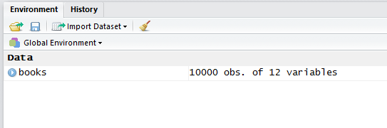
You should now have an R object called books in the Environment pane.

Reading tabular data

read_csv() assumes that fields are delineated by commas, however, in several countries, the comma is used as a decimal separator and the semicolon (;) is used as a field delineator. If you want to read in this type of files in R, you can use the read_csv2 function. It behaves exactly like read_csv but uses different parameters for the decimal and the field separators. If you are working with another format, they can be both specified by the user. Check out the help for read_csv() by typing ?read_csv to learn more. There is also the read_tsv() for tab-separated data files, and read_delim() allows you to specify more details about the structure of your file.

The books CSV loaded as a tibble in your R environment

Discussion: Examine the data

Open and examine the data in R. How many observations and variables are there?

Show me the solution

The data contains 10,000 observations and 11 variables.

• CALL...BIBLIO. : Bibliographic call number. Most of these are cataloged with the Library of Congress classification, but there are also items cataloged in the Dewey Decimal System (including fiction and non-fiction), and Superintendent of Documents call numbers. Character.
• X245.ab : The title and remainder of title. Exported from MARC tag 245|ab fields. Separated by a | pipe character. Character.
• X245.c : The author (statement of responsibility). Exported from MARC tag 245|c. Character.
• TOT.CHKOUT : The total number of checkouts. Integer.
• LOUTDATE : The last date the item was checked out. Date. YYYY-MM-DDThh:mmTZD
• SUBJECT : Bibliographic subject in Library of Congress Subject Headings. Separated by a | pipe character. Character.
• ISN : ISBN or ISSN. Exported from MARC field 020|a. Character
• CALL...ITEM : Item call number. Most of these are NA but there are some secondary call numbers.
• X008.Date.One : Date of publication. Date. YYYY
• BCODE2 : Item format. Character.
• BCODE1 Sub-collection. Character.

Data frames and tibbles

---

Data frames are the de facto data structure for tabular data in R, and what we use for data processing, statistics, and plotting.

A data frame is the representation of data in the format of a table where the columns are vectors that all have the same length. Because columns are vectors, each column must contain a single type of data (e.g., characters, integers, factors). For example, here is a figure depicting a data frame comprising a numeric, a character, and a logical vector.

A data frame can be created by hand, but most commonly they are generated by the functions read_csv() or read_table(); in other words, when importing spreadsheets from your hard drive (or the web).

A tibble is an extension of R data frames used by the tidyverse. When the data is read using read_csv(), it is stored in an object of class tbl_df, tbl, and data.frame. You can see the class of an object with class().

Inspecting data frames

---

When calling a tbl_df object (like books here), there is already a lot of information about our data frame being displayed such as the number of rows, the number of columns, the names of the columns, and as we just saw the class of data stored in each column. However, there are functions to extract this information from data frames. Here is a non-exhaustive list of some of these functions. Let’s try them out!

Size and dimensions

R

dim(books)  # returns a vector with the number of rows in the first element, 
and the number of columns as the second element (the **dim**ensions of the object)
nrow(books)  # returns the number of rows
ncol(books)  # returns the number of columns

Content

To examine the contents of a data frame.

R

head(books)  # shows the first 6 rows
tail(books)  # shows the last 6 rows

Names

R

names(books)  # returns the column names (synonym of `colnames()` for 
`data.frame` objects)
glimpse(books)  # print names of the books data frame to the console

Summary

R

View(books)  # look at the data in the viewer
str(books)  # structure of the object and information about the class, 
length and content of each column
summary(books)  # summary statistics for each column

Note: most of these functions are “generic”, they can be used on other types of objects besides data frames.

The map() function from purrr is a useful way of running a function on all variables in a data frame or list. If you loaded the tidyverse at the beginning of the session, you also loaded purrr. Here we call class() on books using map_chr(), which will return a character vector of the classes for each variable.

R

map_chr(books, class)

OUTPUT

CALL...BIBLIO.        X245.ab         X245.c       LOCATION     TOT.CHKOUT
   "character"    "character"    "character"    "character"      "numeric"
      LOUTDATE        SUBJECT            ISN   CALL...ITEM.  X008.Date.One
   "character"    "character"    "character"    "character"    "character"
        BCODE2         BCODE1
   "character"    "character" 

Indexing and subsetting data frames

---

Our books data frame has 2 dimensions: rows (observations) and columns (variables). If we want to extract some specific data from it, we need to specify the “coordinates” we want from it.

In the last session, we used square brackets [ ] to subset values from vectors. Here we will do the same thing for data frames, but we can now add a second dimension. Row numbers come first, followed by column numbers. However, note that different ways of specifying these coordinates lead to results with different classes.

R

## first element in the first column of the data frame (as a vector)
books[1, 1]
## first element in the 6th column (as a vector)
books[1, 6]
## first column of the data frame (as a vector)
books[[1]]
## first column of the data frame (as a data.frame)
books[1]
## first three elements in the 7th column (as a vector)
books[1:3, 7]
## the 3rd row of the data frame (as a data.frame)
books[3, ]
## equivalent to head_books <- head(books)
head_books <- books[1:6, ]

Dollar sign

The dollar sign $ is used to distinguish a specific variable (column, in Excel-speak) in a data frame:

R

head(books$X245.ab)  # print the first six book titles

OUTPUT

[1] "Bermuda Triangle /"
[2] "Invaders from outer space :|real-life stories of UFOs /"
[3] "Down Cut Shin Creek :|the pack horse librarians of Kentucky /"
[4] "The Chinese book of animal powers /"
[5] "Judge Judy Sheindlin's Win or lose by how you choose! /"
[6] "Judge Judy Sheindlin's You can't judge a book by its cover :|cool rules for school /"

R

# print the mean number of checkouts
mean(books$TOT.CHKOUT)

OUTPUT

[1] 2.2847

unique(), table(), and duplicated()

Use unique() to see all the distinct values in a variable:

R

unique(books$BCODE2)

OUTPUT

 [1] "a" "w" "s" "m" "e" "4" "k" "5" "n" "o"

Take one step further with table() to get quick frequency counts on a variable:

R

table(books$BCODE2)  # frequency counts on a variable

OUTPUT

   4    5    a    e    k    m    n    o    s    w
   1    3 6983   68    3  109    2   21 1988  822 

You can combine table() with relational operators:

R

table(books$TOT.CHKOUT > 50)  # how many books have 50 or more checkouts?

OUTPUT

FALSE  TRUE
 9991     9 

duplicated() will give you the a logical vector of duplicated values.

R

duplicated(books$ISN)  # a TRUE/FALSE vector of duplicated values in the ISN column
!duplicated(books$ISN)  # you can put an exclamation mark before it to get non-duplicated values
table(duplicated(books$ISN))  # run a table of duplicated values
which(duplicated(books$ISN))  # get row numbers of duplicated values

Explore missing values

---

You may also need to know the number of missing values:

R

sum(is.na(books))  # How many total missing values?

OUTPUT

[1] 14509

R

colSums(is.na(books))  # Total missing values per column

OUTPUT

CALL...BIBLIO.        X245.ab         X245.c       LOCATION     TOT.CHKOUT
           561             12           2801              0              0
      LOUTDATE        SUBJECT            ISN   CALL...ITEM.  X008.Date.One
             0             63           2934           7980            158
        BCODE2         BCODE1
             0              0 

R

table(is.na(books$ISN))  # use table() and is.na() in combination

OUTPUT

FALSE  TRUE
 7066  2934 

R

booksNoNA <- na.omit(books)  # Return only observations that have no missing values

Callout

Recall how we use na.rm, is.na(), na.omit(), and complete.cases() when dealing with vectors.

Exercise

1. Call View(books) to examine the data frame. Use the small arrow buttons in the variable name to sort tot_chkout by the highest checkouts. What item has the most checkouts?

2. What is the class of the TOT.CHKOUT variable?

3. Use table() and is.na() to find out how many NA values are in the ISN variable.

4. Call summary(books$TOT.CHKOUT). What can we infer when we compare the mean, median, and max?

5. hist() will print a rudimentary histogram, which displays frequency counts. Call hist(books$TOT.CHKOUT). What is this telling us?

Show me the solution

1. Highest checkouts: Click, clack, moo : cows that type.

2. class(books$TOT.CHKOUT) returns numeric

3. table(is.na(books$ISN)) returns 2934 TRUE values

4. The median is 0, indicating that, consistent with all book circulation I have seen, the majority of items have 0 checkouts.

5. As we saw in summary(), the majority of items have a small number of checkouts

Logical tests

---

R contains a number of operators you can use to compare values. Use help(Comparison) to read the R help file.

operator	function
<	Less Than
>	Greater Than
==	Equal To
<=	Less Than or Equal To
>=	Greater Than or Equal To
!=	Not Equal To
%in%	Has a Match In
is.na()	Is NA
!is.na()	Is Not NA

Callout

Note that the two equal signs (==) are used for evaluating equality because one equals sign (=) is used for assigning variables.

A simple logical test using numeric comparison:

R

1 < 2

OUTPUT

[1] TRUE

R

1 > 2

OUTPUT

[1] FALSE

Sometimes you need to do multiple logical tests (think Boolean logic). Use help(Logic) to read the help file.

operator	function
&	boolean AND
`	`
!	Boolean NOT
any()	Are some values true?
all()	Are all values true?

Logical Subsetting

We can use logical operators to subset our data, just like how we use the square brackets [] for subsetting.

For instance, if we want to extract rows with Total Checkout Number of more than 5:

R

books[books$TOT.CHKOUT > 5, ]

Discussion

Compare the output of the following codes to the previous one:

R

books$TOT.CHKOUT > 5
books[books$TOT.CHKOUT > 5]

What differences did you see in the output?

Key Points

• Use getwd() and setwd() to navigate between directories.
• Use read_csv() from tidyverse to read tabular data into R.
• Data frames are made up of vectors of equal length, with each vector representing each column of the data frame.
• Summarise the dimension, content and variables in a data frame.
• Using the square brackets [] and logical operators to subset data frames.