Reproducible Reports with Quarto
Last updated on 2026-04-22 | Edit this page
Estimated time: 60 minutes
Overview
Questions
- How can I combine my code, results, and narrative into a single document?
- How can I automatically update my reports when my data changes?
- What is Quarto and how does it differ from a standard R script?
Objectives
- Describe the value of reproducible reporting.
- Create a new Quarto document (
.qmd) in RStudio. - Use Markdown syntax to format text.
- Create and run code chunks within a Quarto document.
- Render a Quarto document to an HTML report.
Introduction to Reproducible Reporting
So far, we have been writing code in .R scripts. This is
excellent for data analysis, but what happens when you need to share
your findings with a colleague or a library director? You might copy a
plot into a Word document or an email, then type out your
interpretation.
But what if the data changes next month? You would have to re-run your script, re-save the plot, copy it back into Word, and update your text. This manual process is prone to errors and tedious.
Quarto allows you to combine your code, its output (plots, tables), and your narrative text into a single document. When you “render” the document, R runs the code and produces a polished report (HTML, PDF, or Word) automatically.
Creating a Quarto Document
To create a new Quarto document in RStudio:
- Click the File menu.
- Select New File > Quarto Document…
- In the dialog box, give your document a Title (e.g., “Library Usage Report”) and enter your name as Author.
- Ensure HTML is selected as the output format.
- Click Create.
RStudio will open a new file with some example content. Notice the
file extension is .qmd.
Quarto vs. RMarkdown
If you have used R before, you might be familiar with RMarkdown
(.Rmd). Quarto (.qmd) is the next-generation
version of RMarkdown. It works very similarly but supports more
languages (like Python and Julia) and has better features for scientific
publishing.
Anatomy of a Quarto Document
A Quarto document has three main parts:
1. The YAML Header
At the very top, enclosed between two lines of ---, is
the YAML Header. This contains metadata about the
document.
2. Markdown Text
The white space is where you write your narrative. You use Markdown syntax to format text.
-
**Bold**for bold text -
*Italics*for italics -
# Heading 1for a main title -
## Heading 2for a section title -
- List itemfor bullet points
3. Code Chunks
Code chunks are where your R code lives. They start with
```{r} and end with ```.
R
# This is a code chunk
summary(cars)
OUTPUT
     speed           dist
 Min.   : 4.0   Min.   :  2.00
 1st Qu.:12.0   1st Qu.: 26.00
 Median :15.0   Median : 36.00
 Mean   :15.4   Mean   : 42.98
 3rd Qu.:19.0   3rd Qu.: 56.00
 Max.   :25.0   Max.   :120.00
You can insert a new chunk by clicking the +C button in the editor toolbar, or by pressing Ctrl+Alt+I (Windows/Linux) or Cmd+Option+I (Mac).
Your First Report
Let’s clean up the example file and create a report using our
books data.
- Delete everything in the file below the YAML header.
- Add a new setup code chunk to load our libraries and prepare the data.
Chunk Options
Notice the lines starting with #|. These are
chunk options. - #| label: setup gives the
chunk a name. - #| include: false runs the code but hides
the code and output from the final report. This is great for loading
data silently.
Adding Analysis
Now, let’s add a section header and some text.
MARKDOWN
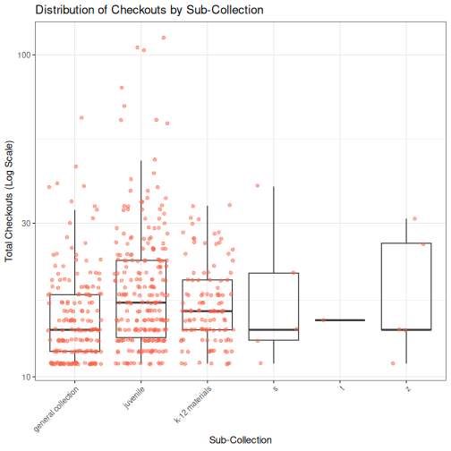
## High Usage Items

We are analyzing items with more than 10 checkouts to understand circulation patterns across sub-collections.
Next, insert a new code chunk and paste the plotting code we developed in the previous episode (ggplot2).
Setting #| echo: false will display the plot in
the report, but hide the R code that generated it. This is
often preferred for reports intended for non-coders.
Rendering the Document
Now comes the magic. Click the Render button (blue arrow icon) at the top of the editor pane.
RStudio will:
- Run all your code chunks from scratch.
- Generate the plots and results.
- Combine them with your text.
- Create a new file named
library_usage_report.htmlin your project folder. - Open a preview of the report.
Challenge: Add a Summary Table
- Add a new header
## Summary Statisticsto your Quarto document. - Insert a new code chunk.
- Write code to calculate the mean checkouts per format (Hint: use
group_by(format)andsummarize()). - Render the document again to see your new table included in the report.
Add this to your document:
```{{r}} #| label: summary-table
books2 %>% group_by(format) %>% summarize(mean_checkouts = mean(tot_chkout, na.rm = TRUE)) %>% arrange(desc(mean_checkouts)) ```
Render the document to see the updated report.
Why This Matters
By using Quarto, your report is now reproducible.
If you download a new version of books.csv next
month:
- Save it to your
data/folder. - Open your Quarto document.
- Click Render.
Your report will automatically update with the new data, creating a fresh plot and table without you having to copy-paste a single thing.
- Quarto allows you to mix code and text to create reproducible reports.
- Use the YAML header to configure document metadata like title and output format.
-
Code chunks run R code and can display or hide
input/output using options like
#| echo: false. - Rendering the document executes the code and produces the final output (HTML, PDF, etc.).
- This workflow saves time and reduces errors when reporting on data that changes over time.